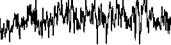
of sine functions. The resulting functions are known as Weierstrass-Mandelbrot functions [227]:

m= E Af rfH sin(2^r f t + 0f), (7.2)

f=-<x

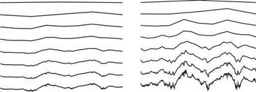
where Af denotes the normal distributed random variable, and r denotes the spatial resolution or lacunarity. 0 is a random phase, and H is again the Holder exponent. The latter determines the ruggedness of the function, as is illustrated in Fig. 7.1.

The second method for synthesizing the fractional Brownian motion uses a sum of bandlimited noise functions [142, 143] whose amplitudes are likewise determined by 1//e, where f is the average value of the frequency of the band – limited functions.[8]

Although there are quite a few different methods for creating noise [52], the optimal noise function should have, if possible, a small frequency range, in order to produce at synthesization the desired 1/fe property. Since, however, a monochromatic function or a function with a very small frequency range cannot at the same time be a noise function, a band limitation is selected [142], such as the Perlin noise function [52, 157].

This type of noise function is defined over a discrete grid, where the function at each grid point is zero, and only between the grid points does has different values. To achieve this, random gradient vectors are defined at the grid points. The function values between the grid points are obtained through linear inter­polation, where the gradient vectors characterize the slope of the function near the grid points.

Because of the zero crossings at the grid points, the synthesized noise function has a fixed lower spatial frequency. Since it might have additional zero cross­ings in between the grid points and saddle points based on the gradient-based syntheses, higher frequencies can develop as well. These are, however, like­wise limited by the linear interpolation. Because of the band limit, the function

has also the advantage of being differentiable in each place, thereby avoiding breaks and creases within rendering. A disadvantage of these noise functions is the occasional surfacing of the grid structure that is caused by the zero values at the grid points. This can be avoided by combining noise functions that accept values different from zero at the grid points [52]. In any case, the Perlin noise function is suitable for approximating the fractional Brownian motion:

n

m = J2 rfH N (tri). (7.3)

i=1

Here, N is a Perlin noise function, and n varies between 3 and 12. The term r is again the lacunarity, and H is a constant, similar to the Holder exponent. If a function has to be evaluated for several variables, then t will be replaced by a vector and a multidimensional version of the noise function is applied.

The third method uses a pure geometric construction, e. g., polygonal subdivi­sion with midpoint displacement. A given set of geometric primitives (usually triangles) is transformed into another, larger set by the application of division steps. In each step, each primitive is replaced with two or more primitives, whereby their number increases exponentially. A similar principle was used with the initiator/generator scheme in Chap. 5, in which the generator replaced the components of the initiator recursively with other components.

Figure 7.2 Division of a line that yields varying roughnesses

If we want to model a one-dimensional Brownian motion, a number of given line segments is refined. Per step, each segment is divided in half, and the respective midpoint is displaced; hereby the midpoint is calculated using

tnew 2(ti + xt+i), (7.4)

Bnew = 2(Bi + Bt+1 )+S(ti+1 — ti)N (tnew )• (7.5)

Similarly to the plant models, here we are dealing again with a procedural description: complex geometry is generated from a base geometry by iterated application of a function. The variables ti may describe locations, the Bi are the “functional” values. Here the function S(At) scales the noise in dependence with the length of the divided segments and thus returns the amplitude factor rfH (see Fig. 7.2).

Saupe shows in [188] that the actual difference between the schemes is the point evaluation. The first two schemes compute the function value f of a

point, without explicitly using the information about the neighboring points. The spatial dependence is here given implicitly over the 1//e property of the sine and noise functions, respectively.

In the last scheme, we needed the positions and/or heights of the neighboring points in order to determine the height of a point to be inserted. In practice, that has far-reaching effects, since most imaging methods, such as raytracing (see Sect. 9.4) synthesize an image by discrete point-by-point evaluation. For such an evaluation, we need the height at a specific point in the terrain, where its definition in the previous scheme (at least the local environment of the point) has to be computed completely. For efficiency reasons, in the last instance, the terrain must also be completely generated in order to then use the geometry for image generation. Due to memory and efficiency reasons this is only possible for limited surfaces.