Examples

After we have described the components and the options of their combination to the p-graph, three examples are used to show how plants are modeled. A sunflower, a rhododendron, and a chestnut tree exemplify the potential of the numerous combination possibilities of components as well as the power of the overall approach.

To model a sunflower, photographs or scanned textures of natural leaves and petal surfaces are needed. With a photo editing program, these are projected onto a transparent background. Here, the so-called alpha-channel, found in standard photo editors, is used, which defines the transparency as an additional

color channel. Usually, for the textures of leaves, only the values zero (com – Section 6.4 pletely transparent) or one (completely opaque) are required. Examples

The picture of the leaf is applied as a texture to the leaf component’s geome­try and a small stalk is attached. Figure 6.7a shows the corresponding p-graph that consists of the icons of the camera, horn and leaf component. Using de­formation values and transformations, the components are parameterized until a natural appearance of the leaves is reached.

In the next step, the leaves are used as branches of a tree component (Fig. 6.7d).

The upper part of the stalk is opened, in order to connect it to the head of the sunflower.

The modeling of the blossom from the seeds and the blossom’s petals are shown in Fig. 6.7b and c. Blossom petals are multiplied with a Phiball com­ponent, whereby the parameterization is selected so that it arranges the petals on a small ring. In a similar way, tiny sticks are multiplied by another Phiball component to produce the seeds of the flower. Both subtrees are attached using child links to the stalk of the sunflower. After further adjusting the parameters, the result is the complete flower.

(a)

(a)

(e)

(b) (c)

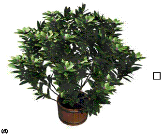
A rhododendron is a good example for modeling a medium-sized shrub. In comparison to the sunflower, the geometric complexity is larger, with approx­imately 30,000 triangles. Here the focus is on the branching structure rather than on geometric properties of the blossoms and leaves.

Again, we will first scan a natural leaf and use it as texture in the leaf com­ponent (see Fig. 6.8a); its p-graph is shown as the upper part of the complete p-graph in Fig. 6.8e. Now a small twig is created. The tip of the twig is built separately, since the leaves of the Rhododendron are set in a special way around the blossom. A phiball component multiplies the leaves and a hydra compo­nent places the blossom leaves inside in the appropriate order (Fig. 6.8b). The

(b)	(c) (d)
Figure 6.10 Maple tree with a total of six branching levels

p-graph now consists of two more components: the phiball to multiply the main leaves and the hydra component to multiply the blossom leaves. Both are joined by the child link with the tree component that will produce the twig.

The production of an entire branch is slightly more complicated: the stems should branch into leaves as well as small twigs. However, to achieve a more realistic shape of a rhododendron shrub, the leaves should not be generated at the position of a twig or vice versa. This is an exception that will be dealt with using the field previously described in the base component. Here some of the branches for leaves are switched off, and instead additional components for the production of small twigs are attached. In the leaf component, only for those branches for which the leaf multiplication was switched off the corresponding switch is turned on. This way, the twig can branch into two different ways (see Fig. 6.8c).

Finally, in the last step, 20 twigs are multiplied using the phiball component. The component is placed somewhat below the ground and thereby phototropism is added to the twigs, which slightly bends them upwards (see Fig. 6.8d).

As a third example, a tree will be created. As already mentioned, the general structure of the p-graph is similar in most trees. A cascade of tree components represents the branching structure, while the leaves, blossoms or needles are attached to the lowest level of tree components.

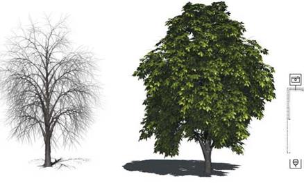
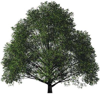
To generate a chestnut tree, as an example of a middle-sized tree, again tex­tures are produced via scanning of a real leaf and bark and then are incorpo­rated into the geometry of a leaf and tree component. If two components are joined and the parameters are set appropriately, a tree as seen in Fig. 6.9a is the final result. For the chestnut tree, a large branching angle in combination with a high gravitropism was configured to produce the main branches. Two additional branching levels are attached and parameterized appropriately. Although it sounds simple, the definition of the parameters especially for the small twigs is still not trivial. The parameters are not independent of each other and cause to some extent a complex interplay. But since the model description can be reused in a very simple way, similar trees can be generated very quickly from an existing model.