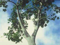
Bloomenthal [17, 18] focuses on the geometrical aspects of tree modeling. The approach is demonstrated with a tree example that shows a branching structure generated by a recursive algorithm. Unfortunately, its production is not revealed. The control points created with the algorithm are then connected by continuous spline interpolation. The surface is created by connecting circular disks that are arranged perpendicularly to the spline.
With previous methods one encounters problems as soon as a natural appearance of branching has to be obtained, which can be seen with Oppenheimer’s approach (Fig. 4.8). Bloomenthal therefore constructs saddle surfaces between the two branching strands that reproduce the natural branching very faithfully. This is illustrated in Fig. 4.9b.
|
|
|
|

(a)
Furthermore, Bloomenthal suggests a modeling method for the roots using so – called “blobs” [16]. Here a surface is defined using the point set that has a given distance to a single geometric object or a quantity of objects. A simple example is a ball whose surface points all have the same distance from the center and are described using the circle equation R2 = x2 + y2 + z2. All points for which the above equation holds are situated on the ball’s surface with radius R around the center point.
For the modeling of branches and roots, the objects that define the surface are the roots’ skeleton curves that diverge in the lower trunk area (see Fig. 4.9b), and so define the root area. The bark is rendered through bump-mapping with a texture that was obtained (via scanning) from genuine bark. The results look very realistic, and the methods can easily be transferred to other trees.


