All point-based methods have in common the need to change their representation at one point back to a polygonal model, which can result in visual artifacts. Rossignac and Borrel [179] try to solve this problem by merging closely positioned vertices within a set of surfaces without being concerned about whether or not they belong to the same surface. This procedure is acceptable for foliage, although the lighting conditions are changing, which leads to artifacts. Nevertheless, the advantage here is the fact that it is still a representation produced with polygons.
A similar approach modifies the geometric description of the foliage without changing the shape of the individual leaves or branches. This method takes advantage of the fact that the shape of a tree has fractal characteristics. Just like in the case of tree skeletons, also the shape of a complete tree is often similar to the shape of a single leaf or to the shape of a small branch with leaves. Hence it might be possible to approximate the foliage of a whole tree with a small set of enlarged leaves. This works at least as long as the tree is displayed at a
large distance. The approach described in the following, we called “Drop and Resize”, attempts to realize this observation.
![]() The type of representation depends here on the overall surface A of the plant as well as its distance r from the virtual camera. If the distance of the image plane to the camera is assigned the value one, the projected overall surface Ai of the plant can be calculated using (see also [207]):
The type of representation depends here on the overall surface A of the plant as well as its distance r from the virtual camera. If the distance of the image plane to the camera is assigned the value one, the projected overall surface Ai of the plant can be calculated using (see also [207]):
1 A
Ai = -. (10.2)
2 r2
Here it is assumed that the triangles are double-sided, where the projection must be calculated with the front as well as the back side. The factor 1/2 takes into consideration the almost random orientation of the leaves in the space, and 1/r2 represents the perspective decrease.
If the original foliage of n leaves should be represented through a reduced set of k uniformly enlarged leaves, then a scaling factor s(k) = )n/k for all the leaves is necessary because of the effective enlargement of the leaves in two dimensions. However, in the practical application we use a weighted form
s(k) = WJ n/k + (1 — w), w Є [0…1], (10.3)
in which w is a factor defined by the user. The weight allows continuous selection between no scaling at all and the correct scaling. No scaling results in a very thin foliage; thus, selecting a medium value often is the best choice.
 |
 |
The deletion rate, which is also defined by the user, displays how quickly and by what function a model is thinned out once the camera moves away. The following images were produced using a deletion rate according to a square function. This kind of deletion rate is motivated by Eqn. (10.2), which describes a square decreasing of the surface in relation to r. Additionally, for each tree a minimal number of triangles is defined, which is used for the minimal representation.
The leaves are deleted on a horizontal plane that is moved vertically through the tree. On the plane, positions are defined and the next leaf is removed. The positions are computed using the already-known function of the Golden Section (Eqn. (3.8)), which is written in polar coordinates (r(i), ф(і)) as
|
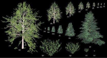
where i is the index of the leaf to be removed, hmax is the maximal horizontal diameter, ph is the horizontal periodicity, and 4п/(v/5+1) is the Fibonacci Angle. If deletion takes place according to this function, then successive positions are never close (see Fig. 3.5). If, however, a random function is used, inevitably clustering would occur, and consequently spots with stronger thinning would result.
The horizontal plane is moved vertically in the tree using a saw tooth or sine function. The sine function has an advantage in that it tends to remove more leaves in the center, where we find the highest concentration, than at the edges of the tree crown.
 |
 |
The periodicity of the sine function usually cannot be seen within an animation, since a vertical period includes several horizontal periods. In Fig. 10.7 the method is used for generating a tree. Here the foliage was reduced from approximately 3500 triangles down to 100 triangles.
If, during the process, the projected surface Ai sinks below the surface of a respective point approximation with a reasonable set of points (see below), then the representation can be switched. Doing so, the described process can be combined with a representation-changing LOD method in order to move the change of the representation into the background and, thus, make it invisible.
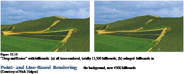
This idea can also be applied to billboards. If a complex forest is to be rendered Section 10.5
using a set of billboards, the number of the billboards can cause problems in Point – and Line-Based
large scenes. In Fig. 10.10(a) we see a scene with a forest that consists of Rendering
13,500 billboards. In the subimage (b), the billboards were enlarged in the
background, and their textures were slightly changed. The visual appearance
essentially remains intact, although still 4500 billboards were used.
(a) (b)
Having discussed several methods, we are now introducing a system that further refines the modeling and rendering with point – and line-based representations. It was proposed by Marc stamminger and George Drettakis together with one of the authors [37]. The system allows even for complex landscapes to be rendered interactively. This is enabled by modern graphics cards with their enormous capacity and efficiency.
Following the open system architecture in Chap. 8, also here single plants are generated as surface models, and are combined with the description of the whole plant cover in the form of an ecosystem data file. As an additional component we now use an LoD editor that approximates the geometry of the plants needed for a fast rendering through points and lines. Generally most of the plant geometry consists of relatively small leaves, which are represented by triangles. Already for a relatively small distance to the plant, for these triangles the average projected surface falls below one pixel, and a representation using a point is more efficient. Similarly, this is true for long objects, such as a stem or the branches of a plant. Also here an approximation using one or more lines is almost faster (see also [231]).
Interestingly with such approximations often also the quality of the rendering increases. Very small polygons most likely start flickering through aliasing effects, due to the graphics hardware’s inability to process high-quality images during animation. Here the rendering of points and lines is essentially more
stable. In fact, an increase in quality is obtained using this kind of approximation.
At the start of an interactive landscape visualization, the rendering system reads in the plant geometries and the ecosystem data. Then from the LOD data of the plants of each ecosystem data file a strongly reduced point set of the total data of all plants is generated. This is done in order to use it once the plants have to be reduced to a level that even one point per plant is too much for an efficient representation. In addition, the ecosystem data can be constructed recursively, meaning a data file can, aside from the plant information, also include references to other ecosystem files. In this way, large areas can be rendered independent of their size, and, what is more, this hierarchical processing of the data enables the user to render such areas in real time.
During the rendering process, the system decides for each plant and each frame to be generated whether the polygonal or the approximated model description should be used. Additionally, the geometric resolution of the approximation is dynamically adjusted to the projected size of the plant. Figure 10.11 illustrates the schematic procedure of the data processing as a partial refinement of the open system architecture of Fig. 8.1.
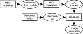 Figure 10.11 System outline for LOD rendering of complex ecosystems


