1.1 Quasi-static analysis
The DCB specimen is made of a unidirectional fibre-reinforced laminate containing a thin insert at the mid-plane near the loaded end. A 150 mm long specimen (L ), 20 mm wide (w )
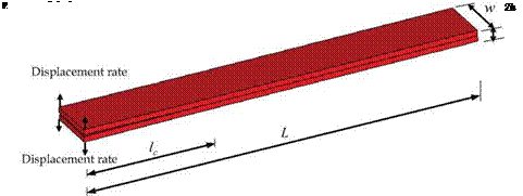
 and composed of two thick plies of unidirectional material (2 h = 2×1.98 mm) shown in figure 5 was tested by Morais (Morais et al., 2000). The initial crack length (lc) is 55 mm. A displacement rate of 10 mm/sec is applied to the appropriate points of the model. The properties of both carbon fiber-reinforced epoxy material and the interface are given in table 2.
Cohesive elements
Case A. 8 elements across the width
Cohesive elements
Case B. 1 element across the width.
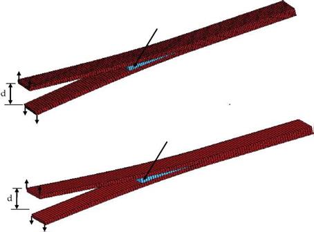
Fig. 6. LS-DYNA finite element model of the deformed DCB specimen
|
Carbon fiber – reinforced epoxy material |
DCB specimen interface |
|
p =1444 kg/m3 |
GIC = 0.378 kJ/m2 |
|
E11 = 150 GPa, E22 = E33 = 11 GPa |
Ko = 3×10⁴ N/mm3 |
|
u12 = u13 = 0.25 , u23 = 0.45 |
ao = 45 MPa case I |
|
G12 = G13 = 6.0 MPa, G23 = 3.7 MPa |
<yo = 60 MPa case II |
|
Table 2. Properties of both carbon fiber-reinforced epoxy material and specimen interface |
The LS-DYNA finite element model, which is shown deformed in figure 6, consists of two layers of fully integrated S/R 8-noded solid elements, with 3 elements across the thickness. Two cases with different mesh sizes are used in the initial analysis, namely: case A, which includes eight elements across the width, and case B, which includes one element across the width, respectively. The two cases are compared using the new cohesive elements with mesh size of 1 mm to figure out the anticlastic effects.
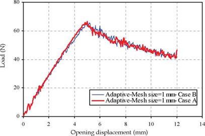
A plot of a reaction force as a function of the applied end displacement is shown in figure 7. It is clearly shown that both cases bring similar results with peak load value of 64 N. Therefore, the anticlastic effects are neglected and only one element (case B) is used across the width in the following analyses.
|
Fig. 7. Load-displacement curves for a DCB specimen in both cases A and B |
Different cases are considered in this study and given in table 3 to investigate the influence of the new adaptive cohesive element using different mesh sizes. The aim of the first five cases is to study the effect of the element size with constant values of interface strength and stiffness on the load-displacement relationship. Different element sizes are used along the interface spanning from very small size of 0.5 mm to coarse mesh of 2 mm. Moreover, cases 3, 6, and 7 are to study the effect of the value of minimum interface strength on the results. Finally, Cases 6 and 8 are to find out the effect of the high interfacial strength.
|
Case 1 |
Mesh size = 2 mm |
oo =45 MPa, Стщіп = 15 Mpa |
Ko = 3×10⁴ N/mm3, Kmln = 1×10⁴ N/mm3 |
|
Case 2 |
Mesh size =1.25 mm |
oo =45 MPa, nmln = 15 Mpa |
Ko = 3×10⁴ N/mm3, Kmn = 1×10⁴ N/mm3 |
|
Case 3 |
Mesh size = 1 mm |
CTo =45 MPa, nmln = 15 Mpa |
Ko = 3×10⁴ N/mm3, Kmn = 1×10⁴ N/mm3 |
|
Case 4 |
Mesh size = 0.75 mm |
CTo =45 MPa, nmln = 15 Mpa |
Ko = 3×10⁴ N/mm3, Kmln = 1×10⁴ N/mm3 |
|
Case 5 |
Mesh size = 0.5 mm |
ao = 45 MPa, CTmln = 15 MPa |
Ko = 3×10⁴ N/mm3, Kmn = 1×10⁴ N/mm3 |
|
Case 6 |
Mesh size = 1 mm |
cro = 45 MPa, amln = 22.5 MPa |
Ko = 3×10⁴ N/mm3, Kmln =1.5×10⁴ N/mm3 |
|
Case 7 |
Mesh size = 1 mm |
cro = 45 MPa, CTmln = 10 MPa |
Ko = 3×10⁴ N/mm3, Kmln = 0.667×10⁴ N/mm3 |
|
Case 8 |
Mesh size = 1 mm |
cro = 60 MPa, CTmln = 30 MPa |
Ko = 3×10⁴ N/mm3, Kmin = 1.5×10⁴ N/mm3 |
|
Table 3. Different cases of analyses |
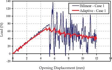
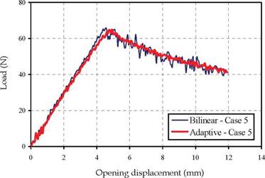
Figures 8 and 9 show the load-displacement curves for both normal (bilinear) and adaptive cohesive elements in cases 1 and 5, respectively, with different element sizes.
|
Fig. 8. Load-displacement curves obtained using both bilinear and adaptive formulations – case 1 |
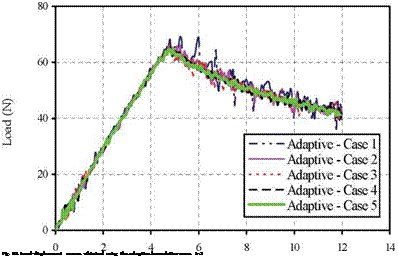
smooth, progressive crack propagation. It is worth mentioning that the bilinear formulation brings smooth results by decreasing the element size. And it is clearly noticeable from figure 9 that both bilinear and adaptive formulations are found to be stable in case 5 with very small element size. This indicates that elements with very small sizes need to be used in the softening zone to obtain high accuracy using bilinear formulation. However, this leads to large computational costs compare to case 1. On the other hand, figure 10, which presents the load-displacement curves, obtained with the use of the adaptive formulation in the first five cases, show a great agreement of the results regardless the mesh size. Adaptive cohesive model (ACM) can yield very good results from the aspects of the peak load and the slope of loading curve if <rmin is properly defined. From this figure, it can be found that the different mesh sizes result in almost the same loading curves. Even, with 2 mm mesh size, which considerable large size, although the oscillation is higher compared with those of fine mesh size, ACM still models the propagation in stable manner. The oscillation of the curve once the crack starts propagates became less by decreasing the mesh size. Therefore, the new adaptive model can be used with considerably larger mesh size and the computational cost will be greatly minimized.
|
Fig. 9. Load-displacement curves obtained using both bilinear and adaptive formulations – case 5 |
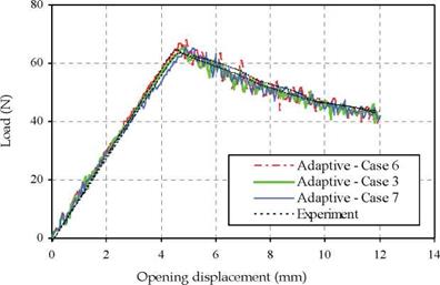
The load-displacement curves obtained from the numerical simulation of cases 3, 6 and 7 are presented in figure 11 together with experimental data (Camanho & Davila, 2002). It can be seen that the average maximum load obtained in the experiments is 62.5 N, whereas the average maximum load predicted form the three cases is 65 N. It can be observed that numerical curves slightly overestimate the load. It is worth noting that with the decrease of interface strength, the result is stable, very good result can be obtained by comparing with the experimental ones, however, the slope of loading curve before the peak load is obviously lower than those of experimental ones (case 7;стш1п=10.0 MPa). In case 6 (стш1п=22.5 MPa) and case 3 ( стш1п =15 MPa), excellent agreements between the experimental data and the
numerical predictions is obtained although the oscillation in case 6 is higher compared with those of case 3. Also, the slope of loading curve in case 3 is closer to the experimental results compared with that in case 6.
Opening displacement (mm)
|
Fig. 11. Comparison of experimental and numerical simulations using the adaptive formulation – cases 3, 6 and 7 |
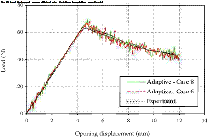
Figure 12 show the load-displacement curves of the numerical simulations obtained using the bilinear formulation in both cases, i. e., cases 6 and 8.
100
![]()
 80
80
g 60
43
<s
о
J 40
20 0
Opening displacement (mm)
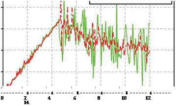
The bilinear formulations results in a severe instabilities once the crack starts propagation. It is also shown that a higher maximum traction (case 8) resulted in a more severe instability compared to a lower maximum traction (case 6). However, as shown in figure 13, the load – displacement curves of the numerical simulations obtained using the adaptive formulations are very similar in both cases. The maximum load obtained from case 8 is found to be 69 N while in case 6, the maximum load obtained is 66 N. The adaptive formulation is able to model the smooth, progressive crack propagation and also to produce close results compared with the experimental ones.

