Review of classical laminated plate theory

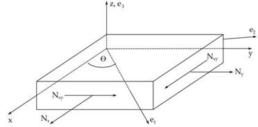
To illustrate the full process of using the self-consistent micromechanics method described herein, two laminate stacking sequences are investigated, the [0/90/90/0] cross-ply laminate and the [45/-45/-45/45] angle-ply laminate. For this example, the laminate level analysis is preformed using classical laminate plate theory but, finite element methods can also be used for more complex geometries and loading conditions.

Consider only the in-plane resultant forces, [Nx, Ny, Nxy] as defined in Figure б, and thermal loading. Under these conditions, Equation 14 gives relationship between the lamina stresses and strains referenced to the principal material axis (i,2).

a, = QjSj (i, j = 1,2,6) (14)

Here, Qij is the reduced stiffness matrix in the material principal coordinate system. Equation 15 shows the entries in the reduced stiffness matrix written in terms of the homogenized stiffness matrix.

Qj = C, j -^^{i, j = 1,2,6) (15)

C33

The stresses and strains can be written in the laminate coordinate system (x, y) obtained by rotating the material coordinate system through an angle, 0, about the material 3 axis, see Figure 6. Equation 16 gives the stress strain relation of Equation 14 written in the transformed coordinate system.

a, = Qij (Ej – ajAT) (i, j = 1,2,6) (16)

A primed quantity is referenced to the laminate coordinate system (x, y). As given in Equation 17, the reduced stiffness matrix referenced to the laminate coordinate system (x, y) is obtained by applying a transformation to the reduced stiffness matrix of Equation 14.

For both the cross-ply and the angle-ply laminates being considered, the in-plane loading is decoupled from any out of plane curvatures. As shown in Equation 18, the laminate strains are related to the force resultants, [Nx, Ny, Nxy], through the extensional stiffness matrix Aij.

{N} = AijSj -{NT} (18a)

Aij= i(Qij) t( and {NT } = AT £[Q’ ](0 {a }()1( (18b, c)

Where the l index sums over the total number of lamina in the laminate and t is the thickness of each lamina. The laminate strains are determined in Equation 19 by rearranging Equation 18a.

* = A – [{N} + {NT}] (19)

For the de-homogenization step, the components of homogenized strain field must be referenced to the principal material axis. This is accomplished by applying the transformation matrix of Equation 17b to the laminate strain in Equation 19. The transformation is applied for each lamina within the laminate. The plane stress condition is then inserted into Equation 2 to determine the out-of-plane strain component, *3 . Equation 20 gives the relationships obtained for an orthotropic material system. The homogenized strain state is now fully specified and the strain state within each representative volume element can be determined.