Modeling Vegetation
The interactive specification of plant associations is necessary in all those places, in which by human intervention the natural development of the plant associations is altered. Some examples are gardens, parks, urban landscapes, and large parts of what we call “cultural landscapes”. Thus the specification encloses many different areas that are dealt with in landscape-architectural planning. As already mentioned above, there are also cases in which one would like to mix explicitly given plant distributions with others that were obtained by simulation. In some cases, particular distributions not controlled by humans have to be studied, such as if a biotope is to be simulated, that after planting is left to its natural development.
Since plants can only in a few cases be positioned individually, efficient specification methods for the modeling of whole populations must be found. in conjunction with this problem, graphical specification proved to be a powerful tool. in this case, the user draws images that are converted afterwards by the system into input data in the form of plant positions and parameters. Similar to the soil factors mentioned above, almost all parameters of plant populations can be specified this way using images.
To specify the density of the population and/or further values such as orientation of the plants or their growth rate, the user paints a grayscale value image. These images can be understood as discrete pixelwise approximation of functions with two variables. Per picture minimum and maximum values are indicated that correspond to the black and white pixels. intermediate values are computed through interpolation:
Here, fmax and fmin are maximal and minimal function values, pmax and pmin maximal and minimal pixel values, and p the actual pixel value.
The conversion of the grayscale values into the positions takes place in the first step. For the production of the points a so-called half-toning algorithm is applied, which is also used in printing techniques for producing grayscale images with discrete black points. There are a number of such methods (for an overview see [221]). For specification of plant distributions, however, only such algorithms are useful that produce uniform points that are varied in their Floyd-Steinberg algorithm ^ density for the production of the gray tone. The Floyd-Steinberg algorithm
[65], a classic in half-toning, provides good initial values for this purpose.
To transformation the grayscale value image into discrete black and white pixels, all pixel values above a given threshold are rendered in white, all others in black. The error made during this process is distributed in both cases onto the neighbors.
7
|
|
|
|
|
|
|
(d)
In Eqn. (8.2) the actual pixel is at the place of the point. The error is distributed to the right neighbor and the three neighbors in the next row. An example clarifies this process: If the threshold has a value of 100 and if the pixel has the value 111, then it is set to 255 (white) and the error amounts to 144; the gray tone of the right neighbor is therefore increased by 144×7/16 = 63, and accordingly for the others.
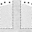
The black pixels generated with this procedure are interpreted as positions of the plants that are to be simulated. Thus, more plants develop in the places that were dark in the gray tone image. After application of the procedure, however, the plants are on a square grid and do not yet have the required distances to each other.
![]() consequently it is necessary to change the positions slightly in a second step in order to obtain random distributed points with almost uniform distances to their next neighbors. This guarantees an optimal covering and also corresponds to the distribution patterns of many species such as grass. The appropriate mathematical distribution again is the poisson disk distribution; hence, the Lloyd method for the adaptive production of such distributions also finds here an application.
consequently it is necessary to change the positions slightly in a second step in order to obtain random distributed points with almost uniform distances to their next neighbors. This guarantees an optimal covering and also corresponds to the distribution patterns of many species such as grass. The appropriate mathematical distribution again is the poisson disk distribution; hence, the Lloyd method for the adaptive production of such distributions also finds here an application.
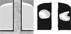
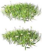
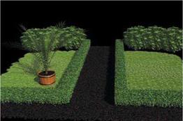
Figure 8.4 shows the entire process of the graphic specification using a part of a garden as an example. The user draws the images for the positioning of the individual species as in Fig. 8.4a. In another image the vigor for the grass tufts in the lawn is defined. To demonstrate the modeling ease, the grass tufts are parameterized in the plant modeling system in such a way that the number of
daisies visualizes the vigor. In Fig. 8.4e, we finally see the result with a palm tree manually inserted. At the positions where a large vigor was specified, many daisies can be seen.

