As already discussed, in our system the vegetation is represented by plant models and ecosystem data files. To deal with the extremely large geometric complexity of entire landscapes, in two ways hierarchical data structures were implemented: firstly for the handling of complex single plants, and secondly for the representation of large amounts of small plants.
The rendering and the LOD treatment of a plant are controlled by Eqns. (10.2), (10.6) and (10.7). These supply in each case the decision for the entire plant, a fact that on the one hand speeds up the production, but on the other hand has also disadvantages. As an example, parts of a large plant such as a complex tree, can be close to the viewer, and for this reason should be rendered as polygons, while other plants are distant and therefore could be approximated.
In order to avoid such an effect, we divide such objects spatially. An octree is produced that divides the object recursively into cells at those places at which much geometric data is present. A similar construction was already addressed in Sect. 9.6 with the quadtrees. These are defined two-dimensionally, while octrees work in a three-dimensional space in an analogous way. For each cell of such an octree, the decision about the geometric representation is made separately by the LoD, and the approximation is executed accordingly.
A similar strategy is pursued for large concentrations of plants. Here it is often too time consuming to handle each single plant, even if only one point of the approximation is used. Consequently, such large sets usually are stored in square cells that are then joined. If there are too many plants in a cell, it is divided until the number of plants is below a given number.
![]()
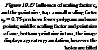 |
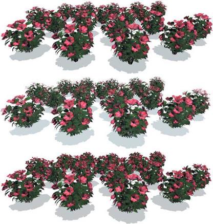 |
Each of these cells is represented using ecosystem data files. Aside from the plant positions, in such a data file also a point set is stored that approximates the whole geometry constituted by the cell. Instead of dealing with single plant models for the rendering, the point set is used when a cell lies in the background of the image. Additionally, cells can be organized hierarchically, meaning ecosystem data files can include several ecosystem data files as references.
In this case the approximations from the references are merged in order to ob – Section 10.5
tain an approximation of the total geometry. Point – and Line-Based
Rendering
Results

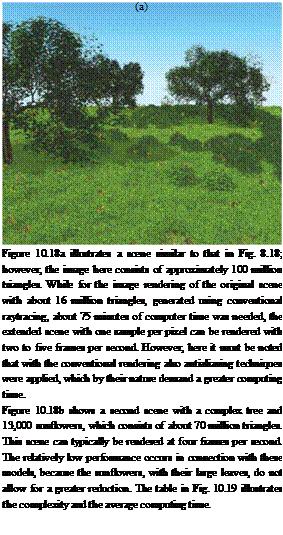 |
|
 |
|
Current PC-based graphics boards offer a true vertex rate of about 5-10 million vertices per second. With the applicable caching strategies that store possibly the most often used geometries of a scene directly on the graphics card itself, a rate of about 11-15 million vertices can be obtained. This data rate is sufficient to render relatively complex outdoor scenes interactively. However, if the current development of graphics boards remains stable for the next two years, then a fluent rendering should be possible for almost all scenes.
After we discussed in the previous chapters a number of approaches to modeling plants and rendering them on screen, in the next chapter of this book the focus will be slightly modified. Up to now we have been dealing with possibly natural and photorealistic images. Now we will introduce nonphotorealistic techniques, though still focusing on the rendering of natural objects.
 Figure 10.19 Geometric complexity of various scenes and the average rates of polygons, lines, and points together with the average frame rate

