The method proposed by Barnsley and Demko [10, 35] for modeling natural objects does not work with geometric data, but rather with two – or higherdimensional point sets. The structures modeled with this method therefore represent only images of the objects, and no surfaces, as was the case in the preceding approaches.
To define an Iterated Function System (IFS) n contractive, affine transformations Mj є R2 ^ R2, M = {M1,M2, • ••,Mn} are required. Each of the affine transformations has six parameters a-f, and is defined by:
щ*,у)=(c d)(x)+(e)• (5.5)
Here point (x, y) is moved to another position. The sequential application of the transformations generates a trace of the point. While the trace is not particularly interesting when applying the transformation only once, amazingly enough complex patterns evolve during the sequential application of several transformations Mj.
The attractor of the IFS is the smallest nonterminal subset A є IR2, so that Mj (p) є A for all p є A and 1 < j < n. The set A always exists and
is unambiguous (see [168]). In order to approximate A, one takes any point ps є A and combines the point sets that emerge if the transformations Mj are applied to the point. If ps is not in A, then due to the contraction characteristics of Mj it is traced back to the attractor.
![]() A can be generated in different ways. Deterministic procedures usually develop a tree, whose nodes consist of points A, and whose edges are applications of Mj. If for each point each function Mj is applied, a binary tree develops for j = 2; for larger values an accordingly broader tree is generated. The tree represents the set of all points producible from one point, and grows exponentially with the number of function applications. Should several initial points exist, then, of course, there will be a tree for each of them.
A can be generated in different ways. Deterministic procedures usually develop a tree, whose nodes consist of points A, and whose edges are applications of Mj. If for each point each function Mj is applied, a binary tree develops for j = 2; for larger values an accordingly broader tree is generated. The tree represents the set of all points producible from one point, and grows exponentially with the number of function applications. Should several initial points exist, then, of course, there will be a tree for each of them.

![]()

In order to produce an interesting image as fast as possible out of this vast set of potential function calls, different search strategies are in place. one of them is the depth-first search, in which, outgoing from the initial point, a function is applied, and following the result, is immediately succeeded by the next. Hence, it is possible to move upward in the tree very quickly. Alternatively, using breadth-first search, for a certain point all applicable transformations are applied. In this way, step by step the complete tree is constructed.
An example of this algorithm is the construction of a Sierpinski triangle. Here for the production of A the breadth-first search is applied, whereby simultaneously an entire point set is processed. Three functions are needed, which in each case have a contraction factor of 0.5 with differing individual displacements of the input points:
|
j |
a |
b |
c |
d |
e |
f |
|
1 |
0.5 |
0 |
0 |
0.5 |
0 |
0 |
|
2 |
0.5 |
0 |
0 |
0.5 |
0 |
50 |
|
3 |
0.5 |
0 |
0 |
0.5 |
50 |
50 |
Figure 5.14 illustrates the result of the application of the functions to a triangular point set. The sides of the triangle are divided by two in each case, and the reduced triangle is moved in three different places.
 To work with balanced trees, defined completely on each level, is a disadvantage if the illustrations Mj contain different contraction rates sj (the so-called Lipschitz constants). These are defined by
II Mj (pi) – Mj (P2) ||< Sj || pi – P2 II V pi, P2 є IR2. (5.6)
For such unequal Lipschitz constants, balanced scanning along the tree leads to an unequal point distribution in A. With an appropriate truncation of subtrees
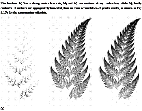
this can be avoided. Figure 5.15a illustrates the effect of the uneven distribu – Section 5.11
tion and the associated visually small convergence. A tree depth of nine and Iterated Function Systems
262,144 points were used in order to assess the following IFS:
 Figure 5.15

Generating a fern leaf with 262,144 points each: (a) deterministic method using a balanced tree; (b) deterministic method with unbalanced tree;
(c) stochastic method
![]() (a)
(a)
Another method introduced by Barnsley [9] consists of a stochastic depth – first search of the tree, whereby a function is selected randomly each time and is then applied. In order to improve the convergence, a similar procedure to that used with nonbalanced trees is applied, meaning that per function Mj a probability Pj "=i Pj = 1, is defined which indicates how of
ten Mj should be applied. If Pj is set according to the Lipschitz constant of the corresponding function, we obtain convergence characteristics as good as those obtained with the truncation method. For the above example, we apply P1 = 0.01, P2 = 0.85, P3 = 0.07, P4 = 0.07. In Fig. 5.15c the result is shown with again 262,144 points.
In his book “Fractals Everywhere” [9] Barnsley extends the method and applies it to simulate images of natural scenes. In such an image many attractors are combined, and also here hierarchical IFSs are used that are not distributing points, but rather whole subimages. The method has the disadvantage that finding appropriate subimages can be a very cumbersome task. Often, only manual intervention yields satisfactory results. If such functions are found, then the attainable compression factors are, however, very high. As an extension of the procedure, if Iterated Function Systems are applied, it is even possible to convert arbitrary input pictures into arbitrary final results.
As an additional extension of this approach, RIFSs (recurrent IFSs) are introduced, in which no arbitrary transformation may follow another, but rather pairs of sequential transformations are specified. This usually is implemented using a graph, whose nodes indicate the transformations, and whose edges denote the possible successor. The attractors of the RIFSs are therefore subsets of the attractors of common IFSs.
Prusinkiewicz and Lindenmayer in [166] describe a procedure for the transformation of L-systems into RIFSs. This is successful if the L-systems describe plants with a strict self-similarity. The reverse, to generate from RIFSs a parametric L-system, is rather simple. Nevertheless, the affine transformations in the parameters must be coded accordingly.


