![]() Each plant is divided into two subgeometries, one is represented by points, the other by lines. The decision on what approximation to use is currently provided by the user. In the future, however, this will be determined automatically through geometric analysis of the model structure. As a further step, the user determines the visual importance of each subgeometry. This is necessary, since some plant parts are visually more important than others. If this effect is exploited, a high visual quality can be obtained with an enormous reduction of the data.
Each plant is divided into two subgeometries, one is represented by points, the other by lines. The decision on what approximation to use is currently provided by the user. In the future, however, this will be determined automatically through geometric analysis of the model structure. As a further step, the user determines the visual importance of each subgeometry. This is necessary, since some plant parts are visually more important than others. If this effect is exploited, a high visual quality can be obtained with an enormous reduction of the data.
The decision with regard to the kind of approximation as well as the visual importance of the plant parts is done once per plant model. Thus in one step all petals of a plant can be allocated a high value in order to increase their visual importance. In the same way they can also be transformed as a whole into a set of points or lines. This assures a minimal manual preprocessing effort.
As already mentioned, compact objects such as leaves are approximated using points. Here two different methods can be applied, depending on whether we are dealing with many small leaves or just a few larger ones. For an amount of many small objects a random point set is used, while for large, complex-
 |
 |
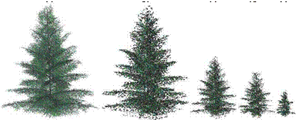
shaped leaves a Poisson disk distribution is applied. Figure 10.12 shows a pine tree whose extremely large number of small needles was approximated using randomly distributed points.
 |
 |
In Fig. 10.13 we see an example for the approximation of a plant with large leaves. If a Poission disk distribution is used, more satisfactory results are obtained. Since the calculation of the point positions is here very complex, previously computed distributions are used. Such distributions can also be generated in a hierarchical form [135]. Thus the appearance remains essentially unchanged, even if through the reduction within the context of the LOD rendering only some of the points are shown.
![]() Thin and long structures are more easily approximated by lines rather than points. Since contemporary graphics hardware renders a line in about the same time as two points, a simple upper bound results for the point approximation. If three or more points can be represented by a line, the line rendering is faster. When four or more points can be represented by a triangle, then this is used instead.[11]
Thin and long structures are more easily approximated by lines rather than points. Since contemporary graphics hardware renders a line in about the same time as two points, a simple upper bound results for the point approximation. If three or more points can be represented by a line, the line rendering is faster. When four or more points can be represented by a triangle, then this is used instead.[11]
Figure 10.14 demonstrates a line approximation. The entire plant is represented by 106 lines. This transformation of the data in combination with the dynamic reduction allows us to render a field with 1500 plants with several frames per second. For rendering the original data consisting of approximately 12 million triangles, an much longer time would be needed.
Using the described system, the LOD data description of a plant contains the polygonal data and its approximation. Beforehand the data was rearranged in
such a way that an efficient rendering and an invisible transition between the polygonal and approximate description are made possible.
|
|
|
|
(a)
The triangle description of the plant is arranged as a whole, but in random order in a display list (a vertex array). The same reordering is then applied to the point and line approximation of these triangles. in this way it is possible to produce any desired approximation by choosing a number k between one and n, where n is the total number of triangles: the first k triangles are rendered normally, and the last n – k triangles are displayed by their point or line representation out of the respective lists (see below).
|
|
|

![]() The best results are achieved if the plants are not uniformly reduced. visually essential parts such as the petals or other elements with special coloring should be reduced later. An example is seen in Fig. 10.15. The daisies in the meadow are visually important, although their geometric complexity is relatively small. if the scene is uniformly reduced, the result is not as good as if the essential parts are not reduced as much. A smaller reduction is often possible without losing much performance, since the visually important parts are often small. Because of the additional storage of point and line data, the quantity of the data to be stored is approximately doubled. Although this is acceptable for the mid-sized landscapes, for larger scenes the entire process of generating point and line approximations must be automated. in this case only a very compact description for the plants can be stored. In the case of Xfrog models this is possible only by storing the production data of the system instead of the geometric data. These are only a few kilobytes. The approximation and production of geometric data would here only be executed on the fly if this becomes necessary during rendering.
The best results are achieved if the plants are not uniformly reduced. visually essential parts such as the petals or other elements with special coloring should be reduced later. An example is seen in Fig. 10.15. The daisies in the meadow are visually important, although their geometric complexity is relatively small. if the scene is uniformly reduced, the result is not as good as if the essential parts are not reduced as much. A smaller reduction is often possible without losing much performance, since the visually important parts are often small. Because of the additional storage of point and line data, the quantity of the data to be stored is approximately doubled. Although this is acceptable for the mid-sized landscapes, for larger scenes the entire process of generating point and line approximations must be automated. in this case only a very compact description for the plants can be stored. In the case of Xfrog models this is possible only by storing the production data of the system instead of the geometric data. These are only a few kilobytes. The approximation and production of geometric data would here only be executed on the fly if this becomes necessary during rendering.
Rendering Section 10.5
Point – and Line-Based
After a plant model and an ecosystem data file have been loaded, the geometric Rendering
data is stored on the graphics board in so-called vertex arrays. These arrays
permit a quick access through the graphics hardware, whereby the program can
control which part of the list is displayed. This decision is made dynamically
for each image during the run time of the system.
First, visibility culling is executed on the basis of the ecosystem data, and in the following it is performed recursively for all visible ecosystem data files on the geometrical plant instances or the hierarchically included ecosystem data files.
once the visible models are defined, then for each model it we determine how it should be rendered. In the following, we are assuming that the original model consists of n triangles T1, …,Tn that in world coordinates have the surface A.
As already mentioned, a part of the set is to be approximated by lines, another part is to be approximated by points. The triangles are divided into two subsets, respectively: TP = Tb…, Tk with the total surface Ap and TL = tk+u.., tn with the surface Ai (we have A = Ai + Ap). Hereby the subset TP should be approximated by points and TL should be approximated by lines. Let us further assume that TL is to be approximated by nl lines L1,…, Lni, TP by Up points Pi,…,Pnv.
In rendering, point and line representations are treated differently: for compact ^ point approximation elements, which are approximated by points, we identify the number of points that are needed to render the object without holes. The number of defined points depends on the total surface of the plant, which was already defined in Eqn.
(10.2), and permits an estimation as to the efficiency of a polygonal or point – based visual representation.
The actual decision can be influenced by the user, in that the user modifies a parameter d’ indicating the distance between two adjacent points in the image plane, i. e., the so-called sampling distance. An increased value of d’ produces a decreased number of needed points and thereby permits a rougher approximation. Consequently the actual size of the points on the screen should correspond to about A’sp = d’2, however, in practice a slightly higher value is used.
The number of necessary points is determined by the projected overall surface of the plant. According to Eqn. (10.2) this is
Here, r is the average distance of the plant to the virtual camera. The necessary point number p is obtained by dividing the projected surface of the plant by the surface of the points:
A’p
p = cp a-г. (1°.6)
Asp
Additionally, for defining the number of points, a factor cp is brought in that permits small corrections for the rendering, and possibly closes still-existing
Chapter 10 holes. Meaningful values for cp are between 1.2 and 1.5. If the number of the Level-of-Detail points needed for the approximation is greater than np, then the object will be
rendered polygonally; otherwise it will be rendered as a point cloud. Further down we show how the number of points is varied and switches between the representations are obtained invisibly.
line approximation ^ For the part of the plant that is to be approximated by lines, the algorithm has to be slightly modified. Here two conditions are mandatory: the projected surface must be represented satisfactorily by lines, and the geometric errors of the line approximation itself should not be too great.
Let L1,Lni be the number of lines for the approximation of TL with a geometric error of el. In the image plane this error will be compared with the sampling distance. If el/r > d’, then TL is rendered polygonally; otherwise, just like in the approximation with points, the projected surface is computed as if all lines were drawn. Here again the projected surface A’l of the triangles TL is determined. The computation is written as follows:
Id’
A’si = l’d’ = —. (10.7)
Here l is the total length of the lines in world coordinates. Accordingly the projected length is l/2r, where the factor 1/2 again considers the random orientation of the lines. The perspective shortening is considered with the factor 1/r, and not, as could be assumed, by 1/r2, since the length and not the surface is projected here. In the next step we define the relationship between the projected surface A’l of the triangle description and the line approximation using
qi = Al/A ‘si. (10.8)
If qi < 1, then ql nl lines are drawn, otherwise the triangles. The lines are here selected randomly just like the points previously.
Up to now we described where and when changes took place between polygonal rendering and the approximation with points and lines. In particular, with large d’, this change can be made visible, and so-called popping artifacts can result. However, in the case of plant models, this can be avoided in that the representations of the whole model are not changed in one single step, but rather continuously for an always-increasing part of the triangles. Since the leaves are equal to many isolated surfaces, this switching is easily possible.
As already indicated above, per triangle two points are randomly defined, and stored in a point list. The triangle list is then randomly reordered, and the per triangle obtained points in the point list are treated in the same way. Both lists are then arranged so that the points for the kth triangle can again be found at the positions 2k and 2k + 1 in the point list; meaning that the first 2k points accord with the first k triangles. The selected degree of detail in each case depends on p. If the necessary number of points p is greater than the triple number of the triangles, the entire triangle set is rendered. This is a good strategy based on the already mentioned ability of graphics adapters to generate a small triangle as fast as three single points.
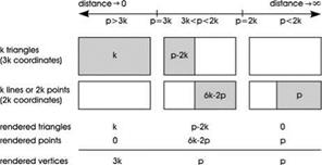
![]() If p < 2k is true, then the first p points of the point set are rendered; for a value of 2k < p < 3k a representation change between triangles and points takes place, in that the first p – 2k triangles are displayed, and simultaneously the point rendering of the leftover triangles. Based on the uniform reordering of the triangles and their point approximation in the preprocessing step, the data can be rendered efficiently using two vertex arrays. This process of data selection is demonstrated in Fig. 10.16.
If p < 2k is true, then the first p points of the point set are rendered; for a value of 2k < p < 3k a representation change between triangles and points takes place, in that the first p – 2k triangles are displayed, and simultaneously the point rendering of the leftover triangles. Based on the uniform reordering of the triangles and their point approximation in the preprocessing step, the data can be rendered efficiently using two vertex arrays. This process of data selection is demonstrated in Fig. 10.16.
 Figure 10.16
Rendering of a plant with points and lines. If the distance is small, polygons will be used. Starting at the distance given by Eqn. (10.6) the polygons are transformed into points. Later only some of the points are rendered.
Because of this form of transition to the approximated rendering, always p vertices are rendered, but never more than 3k. Here the rendering time is directly related to the number of pixels on the screen which were covered up by the object, and is thereby independent of the object complexity. This is an essential condition for efficient rendering algorithms of complex data.
 Figure 10.17 shows the influence of the point size and the scaling factor cp of Eqn. (10.6) on the rendering. If cp is decreased, the elements will be transformed earlier into the points. If the point size is increased, although the spatial resolution is decreased, the size of the points, however, permits a greater reduction. With this form of computation an interesting side effect is obtained: c and the point size can be varied dynamically, in order to achieve a given vertex rate. This in turn allows animations with constant frame rates and a very high frame rate during the pivoting of the virtual camera.


