Data dependent classifiers are based on non-parametric rules. Particularly, the machine learning classifiers use different approaches according to classifier type. In this chapter, largely used non-parametric classifiers were assessed such as ANN, DT and SVM.
The ANN is one of several artificial intelligence techniques that have been used for automated image classification as an alternative to conventional statistical approaches. Introductions to the use of ANNs in remote sensing are provided in (Kohonen 1988), (Bishop 1995) and (Atkinson and Tatnall 1997). The multilayer perceptron described by
(Rumelhart et al. 1986) is the most commonly encountered ANN model in remote sensing (because of its generalization capability). The accuracy of an ANN is affected primarily by five variables: (1) the size of the training set, (2) the network architecture, (3) the learning rate, (4) the learning momentum, and (5) the number of training cycles.
Size of the training set is the most important part in all LUC classifications. If training pixel counts are enough, accuracy of a LUC map would be better than less training pixels.
Network architecture of an ANN is similar to the small part of a neural network (NN) system of human brain. Essentially, there are 3 parts in a NN as input, hidden and output nodes (figure 5). Input nodes are the image bands (e. g. for Landsat TM 6 nodes except thermal band) in a LUC mapping using optical images. Hidden node count depends on the user or previous experiences. There are two way to detect optimal hidden node count; (i) user may check the literature deals with the similar or same area of study site to find the optimal hidden node counts, (ii) user may apply several possibilities itself to find optimal hidden node count checking the accuracy of each applications. According to literature, if a NN system uses the one hidden layer, it is two or three times more than the input nodes generally (Berberoglu et al. 2009). Output nodes counts are equal the class count. Each output nodes are produced a class probability.
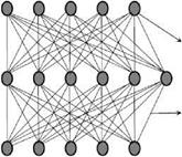 Input layer (image bands)
Node
Hidden layer (various up to input neuron count)
Connections
Output layer (class count)
Fig. 5. NN architecture
The learning rate, determines the portion of the calculated weight change that will be used for weight adjustment. This acts like a low-pass filter, allowing the network to ignore small features in the error surface. Its value ranges between 0 and 1. The smaller the learning rate, the smaller the changes in the weights of the network at each cycle. The optimum value of the learning rate depends on the characteristics of the error surface. Lower learning rates are require more cycles than a larger learning rate.
Learning momentum is added to the learning rate to incorporate the previous changes in weight with the current direction of movement in the weight space. It is an additional correction to the learning rate to adjust the weights and ranges between 0.1 and 0.9.
Number of training cycles is defined according to training error of a NN system. When the training error became optimal, training cycles are sufficient.
In this chapter NN architecture was defined based on previous literature. Berberoglu 1999, designed a NN architecture for Eastern Mediterranean LUC mapping. Several NN architectures were tried in that literature and the highest performance was taken in four
layer architecture. This NN was included 2 hidden layers. First hidden layer was included nodes two times more than input and the second hidden layer was contained nodes three times more than first hidden layer. Learning rate and learning momentum have defined according to training error (table 5).
|
Parameters |
Values |
|
Input layer |
6 nodes |
|
1. Hidden layer |
12 nodes |
|
2. Hidden layer |
36 nodes |
|
Output layer |
11 nodes |
|
Learning rate |
0.001 |
|
Learning momentum |
0.5 |
|
Number of cycles |
44864 |
Table 5. ANN parameters and values
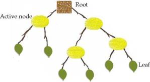
DT is a non-parametric image classification technique. A decision tree is composed of the root (starting point), active node or internode (rule node) and leaf (class). The root is starting point of the tree, active node creates leaves and the leaves are a group of pixels that either belong to same class or are assigned to a particular class (figure 6).
|
|
Fig. 6. Decision tree architecture
A Decision Tree is built from a training set, which consists of objects, each of which is completely described by a set of attributes and a class label. Attributes are a collection of properties containing all the information about one object. Unlike class, each attribute may have either ordered (integer or a real value) or unordered values (Boolean value) (Ghose et al. 2010).
Most of the DT algorithms generally use the recursive-partitioning algorithm, and its input requires a set of training examples, a splitting rule, and a stopping rule. Splitting rules are determined tree partitioning. Entropy, gini, twoing and gain ratio are the most used splitting rules at the literature (Quinlan 1993, Zambon et al. 2006, Ghose et al. 2010). The stopping rule determines if the training samples can split further. If a split is still possible, the samples in the training set are divided into subsets by performing a set of statistical test defined by the splitting rule. This procedure is recursively repeated for each subset until no more splitting is possible (Ghose et al 2010).
In this chapter, gain ratio, entropy and gini splitting algorithms have been used to find the most accurate one, and entropy accuracy was determined almost 3% more accurate than the gain ratio. Gini resulted the poorest performance for the study area. Stopping criteria and active nodes were determined according to fallowing rule;
If a subset of classes determined as pure, create a leaf and assign to interest class. If a subset having more than one class creates active nodes applying splitting algorithm, continue this processes until class leafs became purer.
The SVM represents a group of theoretically superior machine learning algorithms. SVM employs optimization algorithms to locate the optimal boundaries between classes. Statistically, the optimal boundaries should be generalized to unseen samples with least errors among all possible boundaries separating the classes, therefore minimizing the confusion between classes. In practice, the SVM has been applied to optical character recognition, handwritten digit recognition and text categorization (Vapnik 1995, Joachims 1998). SVM uses the pairwise classification strategy for multiclass classification. SVM can be used linear and non-linear form applying different kernel functions. In this chapter only sigmoidal non-linear kernel were used because, model based classifiers have already worked well if data histogram is linear. All data based models were run non-linearly, and sigmoidal application takes less time than other non-linear kernels. Different kernel functions like radial basis function, linear function or polynomial function may be applied. Even the accuracy of the SVM classifier may change when used the one kernel. For example, in polynomial kernel function, accuracy of SVM is various according to applied polynomial order (Huang et al. 2002).
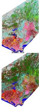
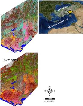
All data dependent classifiers which were introduced in this chapter were evaluated in the Eastern Mediterranean environment (figure 7).

