11.3.2.1 Number of Individuals per Feeding Guild
The percentage of explained variance by the first two axes, using the number of individuals per feeding guild, was 27 % (first axis: F ratio = 1.58, P value = 0.0001), where the marginal effect of the spatial structure of sampled data (PCNM vectors) explained the majority of variance (18 %), followed by the vegetation set (4 %), and last by the landscape set (2 %), whereas the conditional effect explained was 3 % (Fig. 11.2a).
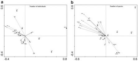
The correlation biplot and correlation matrix resulting from the CCA yielded the following main results (Fig. 11.3a).
1. Overall, the first canonical axis had a strong positive correlation with the PCNM vectors, and with the vegetation variables, whereas there was a weaker association with landscape vegetation variables. The second canonical axis had a stronger positive correlation with stand age, spatial structure of data, structural vegetation variables (e. g., ABa, ABT, ABUNa, SPPT) and SIMP, whereas there was a weaker correlation with landscape variables (see Table 11.3).
|
Fig. 11.3 Distribution of nine avian feeding guilds using (a) number of individuals and (b) number of species. Canonical correspondence analysis (CCA) ordination diagram with feeding guilds (circle) and environmental variables (arrows); first axis is horizontal, second axis vertical. Feeding guilds: BI bark insectivores, CI canopy insectivores, N nectarivores, MCI mid-canopy insectivores, UI understory insectivores, CF canopy frugivores, UF understory frugivores, UG understory granivores, MCG mid-canopy granivores. Vegetation set: AGE stand age, SPPT total species richness, SPPa species richness for adults, SPPs species richness for saplings, ABUNa abundance of adult individuals, ABUNs abundance of all sapling individuals, ABT total basal area, ABa total basal area for adults, ABs total basal area for saplings, Ha mean height of adults, Hs mean height of saplings, TD total density, Da density for adults, Ds density for saplings, SIMP Simpson diversity index, SHAN Shannon diversity index. Landscape structure set: PLAND proportional abundance of each patch type, PD patch density; for landscape configuration: ED edge density at the class level, SHAPE overall shape complexity, ENN patch isolation, TECI fragmentation. PCNM For display purposes the spatial structure vectors are not exhibited in the ordination diagram as well as the samples |
2. Bark insectivores (BI) responded more strongly to the vegetation structure gradient than to the landscape structure, and it can be inferred that higher abundances of BI occurred in older age stands than in younger stands. The latter indicates that the number of individuals of BI increased with successional age (AGE), with the concomitant changes in vegetation structure (e. g., increase in total basal area, basal area, and abundance of adults); in contrast, the abundance of BI decreased with an increase of basal area and abundance of saplings. Moreover, abundances of BI increased as the values of PD decreased.
3. Canopy insectivores (CI) also responded more strongly to the vegetation structure gradient than to the landscape structure. And, similar to BI, the abundance of CI increased with an increase in total basal area, basal area, and abundance of adults, stand age, and moderately by an increase in PLAND, but presented a lower average abundance in comparison to BI.
4. The abundance of nectarivores (N) responded more strongly to the vegetation structure gradient (e. g., stand age, total basal area, basal area, and abundance of adults), rather than to the landscape structure, for which only PLAND had a moderate effect. In addition, the average abundance was lower compared to BI but higher compared to CI.
Correlation matrix
|
Table 11.3 Correlation matrix resulting from the canonical correspondence analysis (CCA) for individual-based and species-based analyses Individual-based analysis Species-based analysis
|
|
Table 11.3 (continued)
|
5. Mid-canopy insectivores (MCI) also responded more strongly to the vegetation structure gradient, and increased with basal area and abundance of saplings, as well as with an increase in SIMP values. In contrast, abundance of this guild decreased with an increase of total basal area and basal area of adults. Specifically, the landscape variables that influenced MCI were PD and ENN, showing a positive relationship.
6. Understory insectivores (UI) showed patterns similar to MCI, responding more strongly to the vegetation variables (increased as basal area and abundance of saplings increased; and decreased with an increase of total basal area and basal area of adults). Landscape variables that influenced positively the abundance of UI were PD and ENN.
7. Canopy frugivores (CF) were positively influenced mainly by stand age and basal area (total and of adults). There was little evidence of quantifiable effects of landscape structure.
8. Understory frugivores (UF) showed an increase in abundance with an increase in the values of TECI and PD, and SIMP; and an increase in abundance with a decrease in basal area (total and of adults).
9. Understory granivores (UG) showed similar patterns to UF: increasing abundance with an increase in TECI and PD, and SIMP, and an increase in abundance with a decrease in basal area.
10. Mid-canopy granivores (MCG) presented higher abundance with an increase in the values of TECI.
11.3.2.2 Number of Species per Feeding Guild
The total amount of explained variance by the first two axes, using the number of species per feeding guild, was 29 % (first axis: F ratio = 1.64, P value = 0.0001); similarly to the individuals-per-feeding guild analysis, the spatial structure of sampling data (PCNM vectors) explained most of the variation (18 %), followed by the vegetation variables (including age) (7 %), and last by the landscape variables (2 %), whereas the conditional effect explained (2 %) (Fig. 11.2b).
The following are the main results from the correlation biplot, resulting from the CCA (Fig. 11.3b).
1. Overall, the first canonical axis had a stronger correlation with the spatial structure of sampling data, stand age, and vegetation variables, whereas in general landscape structure had a marginal negative correlation. The second canonical axis had a stronger correlation with the stand age and vegetation variables, whereas the spatial structure of sampling data and landscape structure had a marginal correlation (Table 11.3).
2. Bark insectivores (BI) were mainly associated with the gradient in vegetation age and structure, indicating that the number of BI species increased with successional age (AGE) with concomitant changes in vegetation structure (e. g., increasing tree height and basal area). In contrast, landscape structure played a marginal role in determining the number of BI species.
3. Increase in the number of canopy insectivore (CI) species was mainly associated with the vegetation gradient (e. g., abundance, density, basal area of adults) and stand age; in general, landscape structure variables (in both first and second axis) had a low overall correlation and therefore played a marginal role in explaining the number of CI species.
4. Increase in the number of nectarivore (N) species was predominantly influenced by an increase in the abundance, density, and basal area of saplings, and by an increase in SIMP, and showed a marginal influence of landscape structure.
5. Mid-canopy insectivores (MCI) responded more strongly to the vegetation structure gradient. The number of species of MCI was positively correlated with basal area and abundance of saplings, as well as with the SIMP values.
6. Understory insectivores (UI) responded to the vegetation structure variables and positively correlated to density and abundance of saplings, but negatively correlated to abundance, density, and basal area of adults.
7. Canopy frugivores (CF) were positively correlated with stand age and the concomitant changes in vegetation structure (e. g., increase in abundance and height of adults).
8. Understory frugivores (UF) showed a positive correlation with basal area of saplings and a fairly marginal correlation with landscape structure.
9. Understory granivores (UG) showed a positive correlation with basal area, abundance, and density of saplings, and a fairly marginal correlation with landscape structure.
|
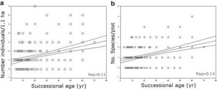
Fig. 11.4 Structural attributes of bark insectivores as a function of successional age: regression models for (a) number of individuals and (b) number of species |
10. Mid-canopy granivores (MCG) were positively correlated to abundance, density, and basal area of saplings and SIMP, but negatively to abundance, density, and basal area of adults.
Stand age was positively related with the abundance (P value = 0.001, R2 = 11 %) and species richness (P value = 0.001, R2 = 14 %) of bark insectivores (Fig. 11.4.), whereas for the rest of the feeding guilds we did not find significant results.


