When modeling larger landscapes, some of the problems addressed in earlier chapters intensify while others become less significant. For example, the arrangement of the objects, contrary to the objects within plant geometries, now basically takes place on a plane; and some subproblems can be solved in twodimensional abstractions, instead having to compute them on the basis of threedimensional data.
The data sets and the complexity of the associated processes force a separation
of the whole process into individual steps, which are connected to a modeling
and rendering pipeline. In such a pipeline, data is produced over several stages, ^ pipeline
whereby each stage is dependent on the previous one for the production of new
data. Here the abstraction level lessens with each step, until finally it ends in
a purely geometrical description of the whole landscape. Following the work
of Reeves and Blau [172], which in the context of a film production dealt with
similar problems (see Sect. 4.5), the procedure is divided into four subareas:
■ Production of Terrain and Soil Factors
Since position and abiotic soil factors such as water and acidity decisively contribute to the development of vegetation, these must be specified in a first step. The terrain is hereby approximated by a height field that indicates an elevation value for each position on the plane. The concentration of resources or the characteristics of the soil can be stored in discrete fields that define a value in regular intervals – for example, in a square grid of a few meters of side length.
■ Specification of Plant Distributions
In the next step the plants are distributed on the height field. For this distribution, methods can be used that are borrowed from plant ecology. Additionally, plant positions can also be the result of a simulation that copies, for example, the competition for light. In places in which ecological systems can develop only to a limited extent due to human interventions, direct specification methods are to be applied.
Modeling of Single Plants
If the positions are known, the respective single plants must be generated. Corresponding methods were already described in earlier chapters. The growth parameters of an individual plant are indicated here by parameters that beforehand were defined within the specification of the plant distribution. At the end of the step, the geometry of the plants is placed in the intended places.
Image Generation
Having the desired geometric data, in the last step single images or animations can be generated. The rendering itself is described in the next two chapters. In this chapter solely the necessary preparatory work on the plant models with respect to reducing their geometric data will be addressed.
Similar pipelines have already been used for the simulation of bird swarms [175], complex phyllotaxial patterns [67], and for morphogenetic production processes [64]. In each of these cases, the simulation and specification were implemented with much simpler objects than the later visualization would have required. Blumberg and Galyean extend this procedure to the interaction of autonomous animated agents in simulation applications [19].
The pipeline structure in this form has also disadvantages. For example, to insert a control loop is a very laborious process: If, during an animation, the number of plants has to decrease because of their competition for light, the corresponding result of the light simulation must be brought back into the simulation for the specification of the plant distribution. In the pipeline then all steps up to the rendering stage must then again be run through. In a practical implementation faster ways would have to be found for efficiency reasons. But since the pipeline structure lends itself to a clear representation for the solution of the entire problem, its principle is maintained in this chapter.
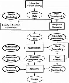
The steps necessary for the pipeline can be divided more precisely into individual modules corresponding to software modules that are combined to form an open system architecture. This architecture resembles here an implemented system that was presented in [39]. Even if some improvements have to be made, the system proved its applicability in handling complex data, as shown by the illustrations in Chap. 9.
The module for terrain modeling produces as an output a file with a height field. This is used together with the soil data as the basis for generating plant positions. The procedures provide in each case a so-called ecosystem file. It contains the positions and parameters of all plants as well as their names. Small plants such as herbs and crawlers are defined here as accumulations. Thus, using the program, for the production of meadows many tufts of grass are manually merged into an accumulation. These are then denoted as a group and assigned a plant name. Later these groups are referenced only as a whole in the ecosystem file, which simultaneously controls the size of the data. Currently some of these tasks are still implemented manually, though, at a later point, they will be automated. It has to be decided, for example, which plants in
Section 8
 Modeling of plant cover
Figure 8.1
Open system architecture for modeling and visualizing ecosystems
a plant association are visually important when characterizing the whole association and therefore should be modeled; which of the plants could be omitted or only suggestively sketched; or if a number of similar biotope types could be, for visual purposes, represented by only one prototype that sufficiently resembles all the others. These preparatory steps are decisive in decreasing the total number of individual plants and associations to be modeled.
![]() The geometry-processing algorithms are more advanced: In order to reduce the quantity of the geometric data, the plant models are quantized. In a meadow, for example, it is not necessary to generate and store each small plant individually. Almost the same visual impression can be produced if a handful instances are individually bent, twisted, and slightly scaled, and are distributed randomly over the meadow. The method for the representation of many individuals by a few instances is called quantization. With this trick the amount of data can often be reduced to a hundredth or even to a thousandth of the original data. Thus for a typical complex scene with 100,000 plants not 10-GByte, but only a 150- MByte memory is needed, an amount of data that can be processed without any problems by modern desktop computers.
The geometry-processing algorithms are more advanced: In order to reduce the quantity of the geometric data, the plant models are quantized. In a meadow, for example, it is not necessary to generate and store each small plant individually. Almost the same visual impression can be produced if a handful instances are individually bent, twisted, and slightly scaled, and are distributed randomly over the meadow. The method for the representation of many individuals by a few instances is called quantization. With this trick the amount of data can often be reduced to a hundredth or even to a thousandth of the original data. Thus for a typical complex scene with 100,000 plants not 10-GByte, but only a 150- MByte memory is needed, an amount of data that can be processed without any problems by modern desktop computers.
Another important step for reducing the data is to work as much as possible with procedural model descriptions. The position information and the actual geometry of the plants should be generated immediately before rendering. Only the data necessary for producing the plant geometry is processed beforehand, which constitutes only a small fraction of the total geometrical data. This advantage was first described by Smith in a work about fractals [201]. It facilitates the handling of the systems substantially.
The quantized ecosystem file is submitted, together with the selected plant representatives, to the rendering system, whose mechanisms are described in the next chapter. In the following we will deal in greater detail with specification
methods for plant distributions. First, direct methods are described, then simulation methods, and toward the end of the chapter the quantization methods for the geometrical data are discussed.


