Reduction of the Geometric Data

The preceding sections focused on the production of individual plant positions and parameters in complex plant communities. For rendering, however, the quantity of the geometrical data must be drastically reduced. The starting point here again is a list L of the plants, which is generated by the simulation models or graphical specification algorithms. L, for example, has the following form:

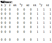
%Descr: % x y z ax ay az sx sy sz vigor domin name 135 279 10 о о 0.0 47.0 1.1 1.1 1.2 1.2 О о Urtica 127 281 11 о о О О 23.4 1.2 1.2 1.2 0.9 со о Urtica 120 271 10 о о О О О о 1.0 1.0 1.0 1.1 о о Poplar

Typically one works with hundreds of thousands of plants, and, without com­pression, L consists of many megabytes. Each line of the list describes a plant of the species (name) with position (x, y, z), orientation (ax, ay, az), rela-

tive size (sx, sy, sz) and relative growth rate (vigor) as well as dominance (domin) by other plants.

For rendering, L is processed line by line, and per plant a geometry production algorithm is called, which generates the geometry of the plant from a previ­ously generated database with all the actual plant parameters (here only the parameters “vigor” and “domination” are shown). Within this process large quantities of geometrical data are produced, also the relatively complex geom­etry production for many plants adds up to unmanageable computing times. The form variety produced with this method – each plant is given an individual appearance – is usually, however, not necessary for the graphical representa­tion. Empirical investigations show that for a good graphical representation of a plant population some few individually bent and easily scaled copies are already sufficient. In the plant community which has to be represented, it is ad­equate to produce per species some representatives, and to distribute replicas at many places in a population. In the illustrations in this and the other chapters therefore we usually worked with 10 to 15 different representatives.

If additionally the number of total species to be represented in the image is limited, some dozen geometric models are usually sufficient to generate the impression of a complete synthetic landscape. The representation of many indi­vidual plants that are copied from a few representatives and are then positioned in many different places throughout the scene is called approximate instancing.

Instancing procedures were already used much earlier for the compact repre­sentation of complex botanical scenes (see [203]). As mentioned before, the general pattern originates from Sutherland [216] and was developed in 1963. A further important step for its use with natural objects was the realization by Smith [201] that the sets of random numbers in stochastic processes for the production of fractal mountains and of particle-based trees can be significantly reduced without incurring visible changes. Hart later developed a procedure for the automatic Instancing of a subset of L-systems [83, 84].

Approximate instancing, the representation of objects using similar objects, was applied for the first time by Brownbill [23] to plant associations. In [39] the procedure was extended to a multidimensional variant that combines the vector quantization with a weighting function (see also [229]). That makes it possible to produce a larger number of representatives for visually important plants.

Back to the list of plants: Within the instancing process, L is converted into a new list L’. This list has the same length, but a significantly reduced number of different objects, since it now no longer refers to individual geometry, but to the representatives. These representatives are stored in a second list R.

To generate the lists, the parameters of the plants of L are divided into two groups. One group of parameters describes position, orientation, and scaling of the plant, and thus can later be generated using an affine transformation of the representative. The other group contains all other parameters.

The list R consists of the descriptions of the representatives. In the next para­graph we will explain how it is obtained. In advance it can be said that the

form of this list is similar to the original list format, only this time all plants are stored in a canonical form, i. e., in the coordinate origin with uniform scaling and orientation. However, the nonaffine parameters of the plant models – thus those of the second group of parameters – are located in this list and are used for generating canonical plant geometry. R has the following form:

vigor	domin	name	rname
1.2	0.0	Urtica	Urtica1
1.2	0.3	Urtica	Urtica2
1.2	0.5	Urtica	Urtica3
0 . 9	0.0	Urtica	Urtica4
0 . 9	0.3	Urtica	Urtica5
0 . 9	0.5	Urtica	Urtica6
1.1	0.0	Poplar	Poplar1

Additonally, each representative receives an explicit name, here stored in the entry “rname”, which is referred by the entities in list L’. When processing R, the geometries of the representatives are generated according to the line entries and stored together with their names.

Now the list L’ no longer refers to an individual geometry. Rather it contains instancing information, which states which representative from R is to be po­sitioned at which place, and how it is to be oriented and scaled. The nonaffine parameters have disappeared out of the list, since they were already used for the production of the representatives, instead the affine transformation is applied to the already created geometry of the representative.

%Descr: x y z ax ay az sx sy sz rname 135.0 279.0 10.0 0.0 0.0 47.0 1.1 1.1 1.2 Urtica1 127.0 281.0 11.0 0.0 0.0 23.4 1.2 1.2 1.2 Urtica5 120.0 271.0 10.0 0.0 0.0 0.0 1.0 1.0 1.0 Poplar1

The advantage of the new data description is not only the smaller amount of the total geometry that has to be produced, but also the increase of the production speed. For setting up a scene only the representatives must be produced in the form of geometry data. The preprocessed geometry is then handed over to the graphics hardware. Now per plant position only one affine transformation is to be produced, instead of having to generate the geometry each time. This type of function can be denoted using homogeneous coordinates using a single matrix multiplication. With the use of graphics hardware, such operations practically do not require any additional time expenditure.

Now we come back to the question of how the appropriate plant representatives can be obtained from the models in L. The answer is a quantization procedure that is found in different implementations in mathematics as well as related fields.