Shape Modeling

Often not only just a species has to be modeled, but rather an individual plant with a particular shape. Examples here are trees growing along a wall or plants deformed under the influence of wind. In both instances, the overall shape of the plant has to be influenced in such a way as to yield a characteristic shape. A total of five mechanisms have been implemented for the modeling of shape. One of the mechanisms is the definition of exceptions within the base compo­nent introduced in Sect. 6.2. The four others are functional modeling, tropisms, freeform deformations, and pruning. These mechanisms will be discussed next.

Chapter 6 As already mentioned in the introduction, while building the temporary i-tree, Rule-Based Object Production component prototypes are transformed into instances, whereby the parameters

are computed individually for each instance, particularly those of the multi­plication components which were stored as parameter ranges. The individual assignment is performed by interpolation, which also permits us to apply a function to the result.

(a)

At this point, random functions as well as other functionally specified parame­ters can be introduced into the system. For example, variations are generated by adding a small random value for the curvature or for the size; for the functional specifications all essential mathematical functions are available.

To parameterize this function meaningfully, a number of variables can be ap­plied in combination with the active value interpolated for the respective in­stance. In this way, positions and orientation, and also recursion depth and the actual iteration number of the instance can be applied.

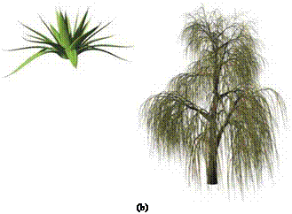
In Fig. 6.11a, an agave plant was modeled using these techniques. Each leaf is individually curved, where the iteration number and a random value deter­mines the curvature. The first generated leaves with a small iteration number are created by the Phiball component at the top of the sphere and thereby re­ceive a small curvature. For the subsequently generated leaves the curvature is increased continuously.

tropisms ^ Tropisms were already discussed in connection with base, leaf, tree, and world components. The modeling with tropisms allows for generating a number of different effects. For the production of a weeping willow, a downward-pointing gravitational field as shown in Fig. 6.11b was applied. If the field is defined in such a way that the directional vectors point towards a center line, and within a cylinder around this line point outwards, then the branching structure can be forced to grow onto a cylindrical shape. This technique was applied to render the philodendron in Fig. 6.11c. More examples are wind simulations, in which

a lateral field is used, and obstructions, which are realized with fields that block the entrance to a space.

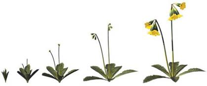In the two foregoing chapters we occasionally addressed the animation of plants. A problem in this area is always the interplay between geometrical and topological changes in the growth of the plant. Prusinkiewicz works with dif­ferential L-systems, in which model changes are described by conventional L-systems; the intermediate growth is generated by differential equations with relatively complex boundary conditions. some of the procedural approaches likewise permit growth of the produced trees, which is due to the limited model palette (mostly simple trees) easier to implement.

With the rule-based object production, we take advantage of the fact that most of the model topology – for instance, how many objects are generated with a multiplication component – is not stored in the topology of the p-graph but as parameters of the components. The topology of the p-graph can therefore be accepted being constant during the process of an animation without too much restriction.

In this case, the parameters which are specified within the components, are understood as parameter sets for a specific time. If different parameter sets are defined for different times, then the values of the parameters for intermediate times can be determined through interpolation. Thus, we are concerned here with a keyframing concept based on parameter values.

Using cascaded keyframing, a local time is implemented. Here one keyframing sequence can be incorporated into another one. If a sequence is produced by a multiplication component during the course of an animation, the local time starts with zero and runs parallel to the global time. In this way, processes such as the opening of petals in a blossom have to be specified only once, and can then be run again at different times and locations independent from each other.

For the cascading of a keyframing sequence, an individual component is used that stores a complete sequence of model descriptions and parameter values at different times. This component is joined just like a normal component to the p-graph of the plant.

A great variety of plants has so far been modeled with this system. The gener­ated trees again consist of a cascade of tree components and have between four

and seven branching levels. The geometric complexity ranges between several Section 6.6 thousand and, as in the case of the maple, several million polygons per plant Animation (see Fig. 6.10).

Figure 6.15 The amounts of time needed for the production of the trees were between one Several models created with the hour and one day for complex trees. Generally modeling expenditure increases system. with the number of branching levels. Thus, if three or four levels are still pro­ducible within an acceptable time frame, a greater expenditure of time must be estimated for large trees not only because of the larger complexity of the data but because of the number of branching levels.

While modeling, the geometrical complexity of the representation can be lim­ited, however, using the exception mechanism from Sect. 6.2 (base compo­nent). For example, all branches except for one can be switched off. The re-

maining branch is then modeled, and only at the end the others again are acti­vated.

In Fig. 6.15 additional models are shown that were generated with these meth­ods. The tree models show the spectrum of different branching structures, and the shrubs are additional examples of average complex models. In the lowest row of Fig. 6.15 various house plants are illustrated, which were likewise cre­ated with this system. These models were transferred after their creation into a professional animation system, which then created the renderings.