Saito and Takahashi [181] recognized the importance of depth-buffer-differences for obtaining important lines. The models they dealt with are, however, smooth surfaces in contrast to the decayed surfaces of foliage. In the same way as discontinuities of the first and second order are appropriate for the production of important lines on smooth objects, discontinuities of zero order, i. e., simple differences, can be used for defining important lines of decayed objects, such as trees and fractals: the contour of a drawing primitive is only drawn if the difference to the depth of the primitive positioned behind it surpasses a threshold defined by the user.
These values can either be defined in the coordinate system of the camera or can be read out directly from the depth buffer. However, the relationship between the two values is not linear. The depth z in the camera coordinate system can be determined from the depth buffer value d (d e [0…1]) using
zi zp (di —dp)
![]()
![]() ___________ zi-zp___________
___________ zi-zp___________
d _ (zi+zp)(di-do) (di+dp) ’
d 2(zi-zp) 2
where d0 and di are minimal and maximal representative values of the depth buffer, z0 is the minimal distance from the virtual camera to the object to be illustrated, and z1 is the distance to the object furthest away (see [136]).
The reason for this nonlinear relationship is the appropriate usage of the available memory for the depth values in connection with the projection of the graphics hardware. Since the values can only be stored with a limited accuracy, this accuracy must be used in a range close to the image plane, where comparatively smaller objects have to be depth-ordered exactly. In the back part of the image, however, where only large objects can still be recognized, the depth test is implemented with less accuracy.
The relationship between the depth in the camera coordinate system and the depth buffer is, after elimination of unimportant terms,
z « l/(d — k),
where l and k are constants that determine the nonlinearity between z and d. The greater the nonlinearity, the greater the relationship between zi and z0. The nonlinearity thereby results in the depth differences for distant objects being smaller than for close objects. Interestingly enough, this effect is often desired. The consequence is that the depth differences between the drawing primitives for distant objects must be relatively larger in the camera coordinate system so that the same difference can be produced in the depth buffer. This way fewer lines and thereby fewer details are produced for distant objects. This effect can also be seen in hand-drawn scenes.
To compute the appropriate threshold for the depth differences in the camera coordinate system, the depth of a tree is defined and an appropriate percentage, such as 10%, is allocated as the threshold. The same happens with depth buffer values: the following examples were computed with values d0 = 0,d1 = 65,535,z0 = 1 and z1 = 11. Here the maximal depth difference of 10 meters accords approximately to that of large trees.
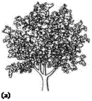
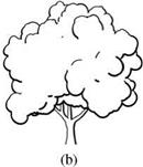 Figure 11.11 Computer-generated drawing of tree I with varying depth-difference threshold and disk sizes: (a) size=0.15, threshold=1000; (b) size=0.7, threshold=2000
In Fig. 11.11, tree I is illustrated with disks as drawing primitives. For varying sizes and depth values different illustrations are yielded for the same object. To enhance the depth impression, each of the lower parts of the primitive contours is illustrated using thicker lines. The trunk and the branches are in these illustrations only represented in a simple way by their outlines.
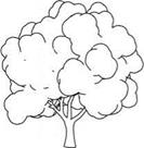
![]() The implementation of additional drawing primitives is shown in Fig. 11.12. Here the example tree II is illustrated using leaf-shaped primitives with an outline depending on the normals of the respective leaf positions selected from the given set. For the definition of the respective leaf shape, interpolation between nine given primitive outlines takes place.
The implementation of additional drawing primitives is shown in Fig. 11.12. Here the example tree II is illustrated using leaf-shaped primitives with an outline depending on the normals of the respective leaf positions selected from the given set. For the definition of the respective leaf shape, interpolation between nine given primitive outlines takes place.
This procedure offers another advantage: because of the interpolation, the variation of the leaf shape can be applied to a greater or lesser degree, and it is possible to replicate the different representational forms for the structure, ranging from an almost flat to a three-dimensional appearance.

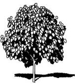 Figure 11.12
Application of leaf-shaped primitives; here interpolation takes place between nine given shapes depending on the direction of the normal
 |
|
 |
 |
 |
|
As already mentioned, through the nonlinear representation of the values in the depth buffer, an automatic reduction of the detail for trees in the background is possible. This effect can be increased or decreased by varying the relationship between z1 and z0: a small quotient produces smaller differences, a larger one allows for the trees in the background to only appear as their outlines.
 This kind of visual abstraction can be reinforced by scaling the primitives for the plants in the background. Kowalski et al. propose in [111] an equation for the scaling factor r for the size of their primitives: it uses a weighted sum between a scaling d/s for primitives with visually constant size in all distances (here d is the desired projected size, and s the actual size), and a scaling with uniform size:
r = w(d/s) + (1 — w) w Є [0.. 1] (11.2)
Equation. (11.2) can be extended in that w is allowed to accept values larger than one, and in this case the second term can be eliminated. The result is that the primitives for the more-distant trees can become greater, and in this way an additional abstraction degree is created. Figure 11.13 shows the effect. in part (a) tree i is illustrated with different distances to the viewer, where the primitive size was not modified. In part (b) the primitive size was enlarged over-proportionally, so that the trees behind the first tree appear to be smoother.
There are three application scenarios from architecture and landscaping in which the production of hand-drawn plants is not feasible or not even possible. In the first case individual high-quality illustrations are to be produced from computer-generated planning data, in order to make the planning results visually accessible for the user. Here it is a special advantage if the plants can be illustrated realistically as well as at different abstraction levels, since here the illustration of the landscape can be adjusted to the needs of the planner.
 In the second case, a planned landscape or a building with surrounding plants is to be animated as a drawing, so that the viewer can virtual stroll around. For this, the produced images must inherit a large coherence in order to avoid flickering during the animation.
 In the third case, a planned area is to be interactively explored. This can also be implemented using a drawing-like style, which has the advantage that many details can be left out, though simultaneously the planning-like character is visualized. In this case the images must be rendered very quickly, and loss of quality is here acceptable.
The rendering process therefore consists of two variants. The first variant produces images with high quality, where the computing time can be higher; in the second variant a quick rendering with lower quality is desired. Both variants are realized within the framework of the software. The results are discussed in the next section.
In the first step the depth differences must be computed. For interactive usage, the tree skeleton is illustrated together with the abstract drawing primitives, the depth buffer is read out, and all pixels with a depth difference beyond a given threshold are colored black. The resulting image can be combined directly with other elements in the scene. For high-quality images, and also animations, tree skeletons and leaf primitives are treated separately. The images are later combined. Here for each image part, an individual depth-difference threshold is used.
shadow computation ^ Many of the drawing styles require the illustration of shadows. As already indicated in Chap. 9, this can be implemented in two ways: In the first method, each pixel can be calculated via the software to analyze whether the illustrated object is illuminated directly from the light source or whether another object lies in between. In this method the image is generated from the viewing direction of the light source, and the depth buffer is read out. In the second step, if the coordinates and the depths of the objects are transferred into the coordinate system of the light source, with the support of the stored depth buffers, it can be determined whether an object is closer to the light source. In this case the object lies in the shadow (shadow buffer technique).
The second method uses the graphics hardware. Each triangle of the scene produces together with the light source a shadow volume. Per triangle a frustum of a pyramid with a triangular base is created. With a special buffer, the light source for all objects within this volume is switched off [136]. The method has
 the advantage, facilitated by the graphics hardware, of working very quickly. Section 11.3
Because of some additional technical constraints it unfortunately does not work Synthetic Plant Drawings
with the large number of isolated surfaces that are found in the foliage of the
trees.
Consequently, the shadows for the plant sketches are calculated by applying the software method. The respective image will be stored in a separate shadow buffer, and can then be used for the modulation of the depth threshold or to modify the line thickness of the illustrated primitives. In an interactive case, no shadows are computed at all.
 |
 |
|
For rendering high quality images with temporal coherence, the retrieved pixels above the depth-difference threshold are not drawn directly, but instead are transferred into lines (vectorization). Here a so-called mean-square-error method [155] is applied, which inserts a fitting line or a curve segment into a set of points. The vectors produced can then be drawn with different line styles, and can also be scaled as needed.
An additional refinement of the procedures uses an index image with false color representation (see Sect. 9.8). With the subsequent vectorization, all the primitives belonging to the lines can be combined and drawn later. This increases the quality of the illustration immensely. Also the coherence can be noticeably increased, for example if an object has to be turned and scaled. An additional enhancement of the quality could be achieved if for each of the primitives the respective visible area of the outline was assigned, and then interpolated over time. This would eliminate even the last remaining artifacts in the animation, although the image sequences already reflect a high quality without this optimization.
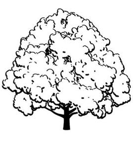
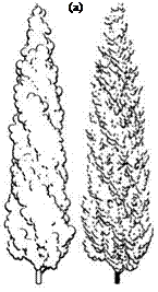
In Fig. 11.14a, the thuja from Fig. 11.9 is illustrated using two different drawing styles. In both cases ellipses were used as drawing primitives, here with
Chapter 11 random orientation. During the drawing a slight random move and rotation Landscape Sketches was executed, so that the lines are overlapping, which gives the image a lighter
appearance. While for the left thuja the above algorithm with a threshold of 400 was applied, the right version was created through a slight modification: here each time only the lower part of each visible ellipse was drawn. The threshold was decreased to a value of 100.
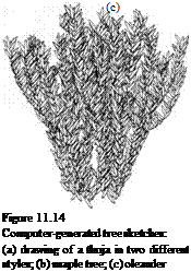
The maple in Fig. 11.14b consists of 16,200 primitives and is rendered from part (a) just like the thuja. The threshold here has a value of 1000. For the rendering of the oleander in part (c), leaf-shaped primitives with random orientation were used. A threshold of 10 assures that practically all visible parts are drawn.
The illustrated results were published in [42]. Although the method is a partial success on the way of rendering computer generated plant sketches, with this procedure only a small part of the wide range of drawing styles can be replicated. The method does however allow for a certain freedom in generating variations, so that a variety of images within a presentation can be rendered. interactivity ^ Unfortunately, the method in the present form has only a limited suitability for an interactive rendering. The readout of the depth buffer is a time-critical operation that currently is still not sufficiently fast. New forms of hardware-related programming of graphics boards could here lessen the problem. These, for example, allow for rendering routines such as the retrieving of depth differences directly in the graphics memory without having to transfer the data to the cpU. The suitability of this method for synthetic illustrations must however still be evaluated.
The following paragraphs focus on additional questions with regard to the rendering of drawn plants, and also on more common objects. We address the rendering of cross-hatchings that are found in various drawing styles. The implemented methods allow for an automated rendering of cross-hatchings on different surfaces. Two of the methods are introduced in the following.

