Design formulae

The fracture energy, rF, depends on both the strength properties of adherents, concrete and adhesive, and the properties of the concrete surface. When the reinforcement is correctly applied, the detachment of the reinforcement occurs with debonding in the concrete layer and the specific fracture energy of the interface law can be written in a form similar to that

used for the shear fracture (mode I). Therefore, in order to obtain design formulae, the fracture energy can be expressed as a function of the shear strength in the concrete: rF(xb, max), where Tb, max depends on the tensile and compressive strength of concrete.

4.1 Theoretical formulations of debonding load

In most formulations the fracture energy is directly expressed as function of the tensile and/or compressive strength of concrete and it is also function of a shape factor depending on the FRP to concrete width (bf/bc).

Based on experimental tests, many theoretical formulations have been proposed in the past (Taljsten, 1994; Neubauer and Rostasy, 1997; Brosens and Van Gemert, 1997; fib bulletin, 2001; Chen and Teng, 2001; Smith and Teng, 2002; CNR-DT200, 2004; Lu et al., 2005; Seracino et al., 2007) to evaluate bond strength at the end of R. C. beams externally strengthened with FRP.

The lay out of the existing formulations is often similar; the differences are essentially related to the numerical coefficients calibrated on experimental results and to the eventual presence of safety factors. This last point is an important issue in using these formulations for design when the safety level (mean, characteristic or design provisions) has to be chosen. Some of these formulas are used to predict the bond strength at the intermediate crack too, through the exchange of some factors (Teng et al., 2003; Chen et al., 2006; CNR-DT200, 2004). For illustrative purposes an example of a calibration procedure of a simplified design relationship based on experimental data is reported in the following section. The example was made with reference to the theoretical relationship (67) suggested in CNR DT200-2004 but the procedure can be used to calibrate also different formulations.

N 1	’ Pl * bf * VkG * kb V2 * Ef * tf * Vfck * fctm 1 Ef * tf	(67)
1 M, max I—————– Y f, W Y c
	L = f f e 2 * fctm	(68)
	kb = I2 – bf/bc b 1 + bf/400	(69)
H2 -1)	if Lb < Le; Pj = 1 otherwise	(70)

fck being the characteristic value of cylindrical compressive strength of concrete, kG a coefficient regarding the experimentally calibrated fracture energy and equal to 0.064 for mean value provision or 0.03 for design value. The safety factor for debonding failure, yf, d, is usually assumed equal to 1.2 or 1.5 (non-controlled or controlled gluing application); yc is the safety factor for concrete (equal to 1.5, EC2, 2004).

on experimental data through a probabilistic approach, as suggested in (EN1990 – Annex D) and applied by Monti et Al. (2009).

By assuming a simplified formulation similar to the design relationship (67), taking into account no safety partial factors, the debonding strain can be expressed as:

where the coefficient kbf can be calibrated based on experimental results using a least-square procedure consisting in the resolution of the following minimum problem (Bilotta et al. 2011):

Furthermore, a random variable 8 can be defined, for each ith test, as the ratio of the experimental debonding strain, eexp, i, to the theoretical one, efd, i, evaluated by considering the geometric and mechanical data characterizing that test:

s

8, =-^± . (73)

sfd, i

The error function, 8, can cover the uncertainties of the simplified model considered as follows:

Sfd =Sfd (kbf, fc, fct, Ef, tf, bf, kb )’8 , (74)

therefore, the mean value of the intermediate debonding strain can be obtained by a coefficient km, starting from kbf adjusted by means of the mean value of the error parameter 8 , being in general 8 Ф 1 because the regression line is imposed to intercept the origin:

km = kbf -8 . (75)

Obviously, this strain is proportional to the debonding stress, being linear elastic the FRP constitutive law.

If the random variable represents a strength, its characteristic value is often defined for design purposes as the 0.05 percentile of the frequency distribution associated to the examined variable. Gauss distribution is the most generally considered for describing the errors. Assuming that the Young modulus of the FRP reinforcement, Ef, and the concrete tensile and compressive strengths, fctm and fcm, are the only mechanical parameters influencing the value of the maximum axial strain developed in FRP at debonding, the expressions for the both general model and the calibrated one involving the coefficient kbf as well as 8 are:

Sth, m = 6th, m (Ef, fcm, fctm , S, kbf)- (77)

Ef, fc and fct are assumed normally and independently distributed random variables, with a priori values of the coefficients of variation according to the design relationships provided by codes and literature information (Bilotta et al. 2011). Also the variable S can be assumed as normally distributed. However, the hypothesis of normal distribution is required to be checked at least by comparing the experimental curve of the cumulative frequency to the theoretical one corresponding to a Gaussian distribution having the same mean value and standard deviation. Hence, under the hypothesis of normal distribution for the variable S, the strain provision corresponding to the 0.05 percentile of the Gaussian distribution is:

6th, k = 6th, m – 1.64 •[Var(6th, m)] °’5

where the variance of £th, m can be expressed as:

Var (Sft, m) = CEfm • Var (Ef) + • Var (fcm) + • Var (fctm) + C2m • Var (Sm)

d6th, m	, f =	d6th, m	, Cfctm	d6th, m	, Cfctm	d6 th, m
dEf	df	df.	58
Ef		fcm		fctm	m

CEfm =

If the Eqs. (80) and (79) are substituted in the Eq. (78), the following general expression is obtained, providing the 0.05 percentile of the debonding load:

6th, k = 6th, m -1.64 • 6th, m • [a • CoVf + b • CoVfcm2 + c • CoVw2 + CoVSm2 ]0-5

where the coefficient a, b, c depend on the functional relationship of Ef, fcm and fctm in the expression of Bth’, moreover the coefficients of variation are defined for each parameter as the ratio of the mean value to its standard deviation:

Clearly the coefficient of variation of the variable Sm, CoVgm, depends on the data distribution. The Eq. (81) can be written as:

assuming:

kk = km • (1 -1.64 • [a • CoVEf 2 + b • Cof2 + c • CoVw2 + CoV5m 2 ] ^). (84)

The use of percentiles lower than 0.05 can be alternative to the use of safety factors that usually have to be additionally applied to characteristic provision to take into account the model uncertainness (EN1990 – Annex D).

In Table 2 the coefficient km and the R2, that is a measure of the reliability of the regression, are reported: two different experimental samples were considered for sheets and plates respectively. Note that for the cured-in-situ FRP systems (sheet) the R2 value is quite high (0.855); on the contrary for the preformed systems (plate) the R2 value is quite low (0.349), mainly due to a higher scattering of the experimental data.

In addition the mean value of the variable 8m and its CoV are reported. In both cases the CoV, that represents a measure of the model significance, is lower than the threshold value of 40% (Monti et al., 2009) so that all the models can be considered reliable.

Finally, Table 2 shows that different scattering of experimental data leads to very different 0.05, 0.005 and 0.001 percentile of the calibrating coefficient k, for sheet and plate respectively.

FRP type	km	R2	sm	CoVS Sm	km ‘Sm	kk,5%	kk,0.5%	kk,0.1%
Sheet	0.270	0.855	1.027	17.7%	0.278	0.192	0.143	0.117
Plate	0.236	0.349	1.064	23.2%	0.251	0.152	0.095	0.064

Table 2. Statistical data

0.012

s

0.010

0.008

0.006

0.004

0.002

0.000

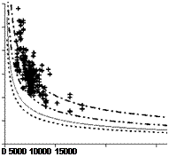
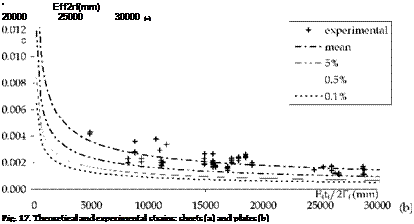
Theoretical debonding strain (71) are plotted in Fig. 17a, b versus the parameter Eftf jkbyJfcmfctm , for sheets and plates respectively. Each curve is obtained with reference to

each percentile of the k coefficient reported in Table 2. Theoretical debonding strains, obtained by means the calibrating procedure showed above, can be easily compared with experimental ones (singular point).

5. Conclusions

A wide overview of the key contributions in understanding the mechanical behavior of FRP laminates bonded on a concrete substrate has been reported in this chapter. Several original contributions have been also proposed.

First of all, a general analytical model has been formulated for describing the distribution of shear and normal stresses within the adhesive layer connecting the FRP laminate to the substrate. The key dimensionless parameters governing such distributions have been clearly pointed out and their influence has been showed in numerical application. The possible simplification of that general analytical model in a simpler one based on the assumption of a layer of elastic springs connecting the FRP laminate to the substrate has been also proposed. This model leads to much simpler differential equations with a reasonable reduction of accuracy. Moreover, it can be easily extended to the nonlinear branch, especially in the case of a supposed bi-linear (namely, elastic-softening) behaviour of the interface in terms of relationship between shear stresses and interface slip. Closed-form solutions of the stress and strain distribution throughout the FRP laminate can be derived under this assumption.

Those closed-form solutions can be employed for identifying the actual properties of the interface relationship. The numerical stability of an indirect-identification procedure based on those solutions has been demonstrated in the section 3 of this chapter. Moreover, it has been showed that the experimental data can be simulated with good accuracy even if a simplified adhesion law (i. e. a bilinear adhesion law) is assumed.

The values of the mechanical properties of the adhesive FRP-to-concrete interface obtained by some experimental tests available in the scientific literature have been finally utilized for calibrating simplified design-oriented formulae for determining the values of the maximum axial strains which can be developed in the FRP laminate before the onset of the debonding phenomenon. The effect of both the material randomness and the model uncertainties in defining the characteristic value of the axial strain in FRP at debonding have been handled by means of a well-established statistical procedure.