Interpreters classify (LU/LC) easily by using image tone (color) and texture (Campbell 2002; Lillesand et al. 2007). The color of A. formosana was similar to that of other vegetation in some regions, so the texture was used to extract data for this species more effectively. Many speckle reduction filters (e. g., Lee, Lee-Sigma, Frost) assume a Gaussian distribution for speckle noise (Lee 1981; Frost et al. 1982). The maximum a posteriori (MAP) filter is used to attempt to estimate the original pixel digital number (DN), which is assumed to lie between the local average and the degraded (actual) pixel DN. MAP logic maximizes the a posteriori probability density function with respect to the original image (Frost et al. 1982). However, a recent study has shown this to be an invalid assumption.
|
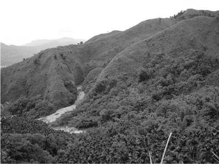
Fig. 18.2 ilar distribution of Arundo formosana |
Natural vegetation areas have been shown to be more properly modeled as having a gamma-distributed cross section. A textural image was created using 3 x 3 pixels and a moving window gamma filter. We established the distribution of A. formosana with color and texture.
Image classification is the major task of remote sensing (RS), including image analysis and pattern recognition. The maximum-likelihood classifier (MLC) of supervised classification provides higher accuracy assessment than minimum distance to means classifier, parallelepiped classifier, and unsupervised classification methods (Giannetti et al. 2001; Boles et al. 2004; Lillesand et al. 2007). Classification error matrix is one of the most common ways to express the classification accuracy of an image. Its overall accuracy can be assessed with the kappa coefficient (K), which is a calculation of agreement or accuracy for LU/LC classification (Congalton 1991; Congalton and Green 1999). The result of a kappa analysis is computed as follows:
r r
N^2 nii -^2 (nt+ x n+i)
k = —= 7J=1 (18.1)
N2 – (ni+ x n+i)
i=1
|
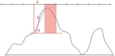
Fig. 18.3 Illustration of the hypotenuses in slope surfaces of different spatial scales: a = adjacent (read from RS data), b = hypotenuse, and в = slope degree (obtained from raster image) |
where r is the number of rows in the matrix, nu is the number of observations in row i and column i, ni+ and n+i are the marginal totals for row i and column i, respectively, and N is the total number of observations (Bishop et al. 1975). This accurate assessment has been recognized as a useful tool in judging the fitness of remote sensing data. Janssen and Vanderwel (1994) pointed out that it should be higher than 0.7 to ensure a good classification result.


